About the Benchmark
This page is not intended to be a tutorial or an in-depth documentation of the benchmark. The goal here is to provide a good overview over what the benchmark covers as well as intuitions on how the different parts work and what to expect from them. For a more technical explanation of the benchmarking code, please refer to the documentation.
- Features - Overview
A non-exhaustive overview of the features of the benchmark. - Surrogate Models
An overview of the surrogate models that are currently implemented to be benchmarked. - Data
An overview of the datasets that are currently included in the benchmark. - Modality
A full account of the different modalities that can be run in the benchmark. - Training
Explanation on how the training process works and how to configure it. - Benchmarking
Explanations on how the benchmarking process works and how to configure it.
Features
A non-exhaustive overview of the features of the benchmark.
Baseline Surrogates
The following surrogate models are currently implemented to be benchmarked:
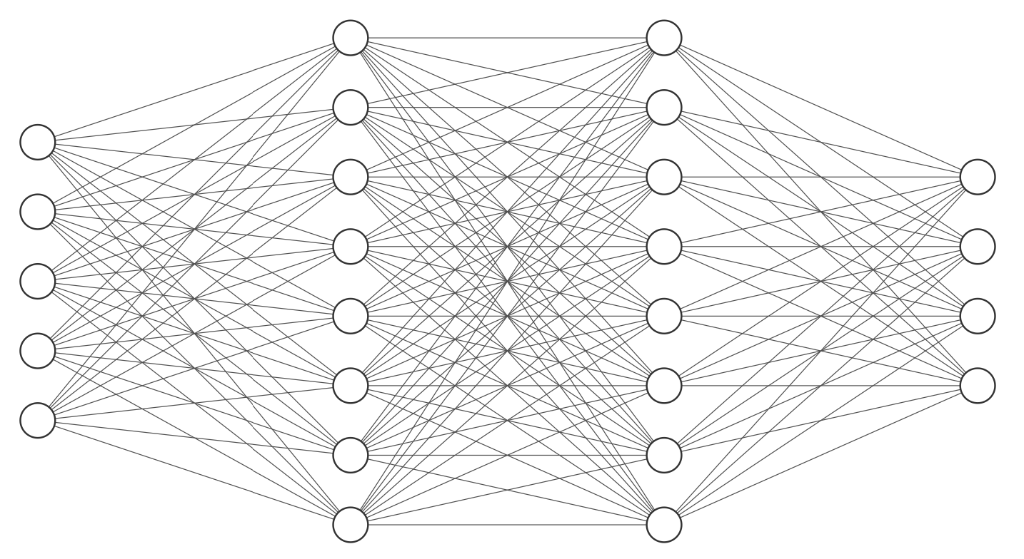
- Fully Connected Neural Network: The vanilla neural network a.k.a. multilayer perceptron.
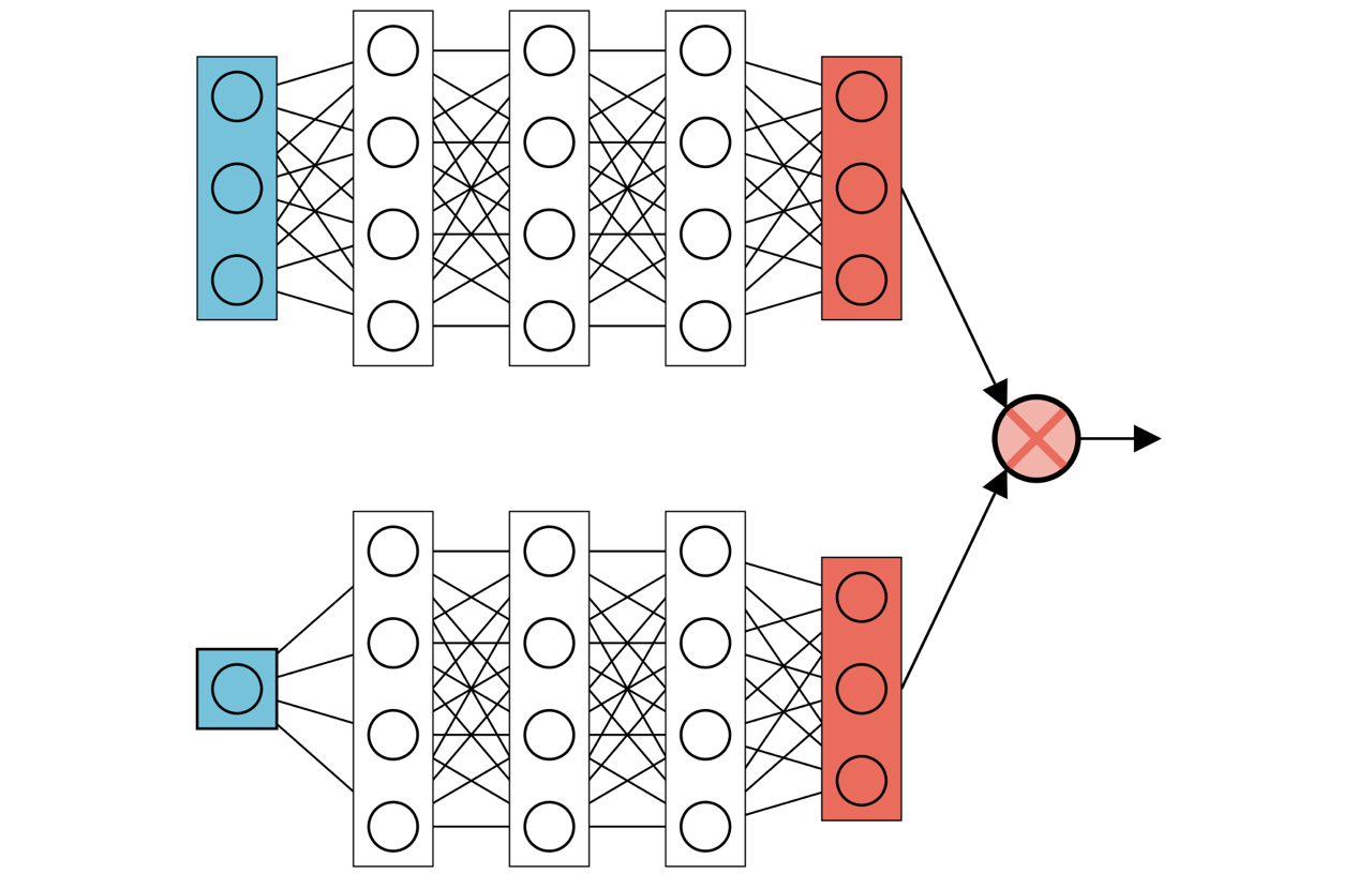
- DeepONet: Two fully connected networks whose outputs are combined using a scalar product.
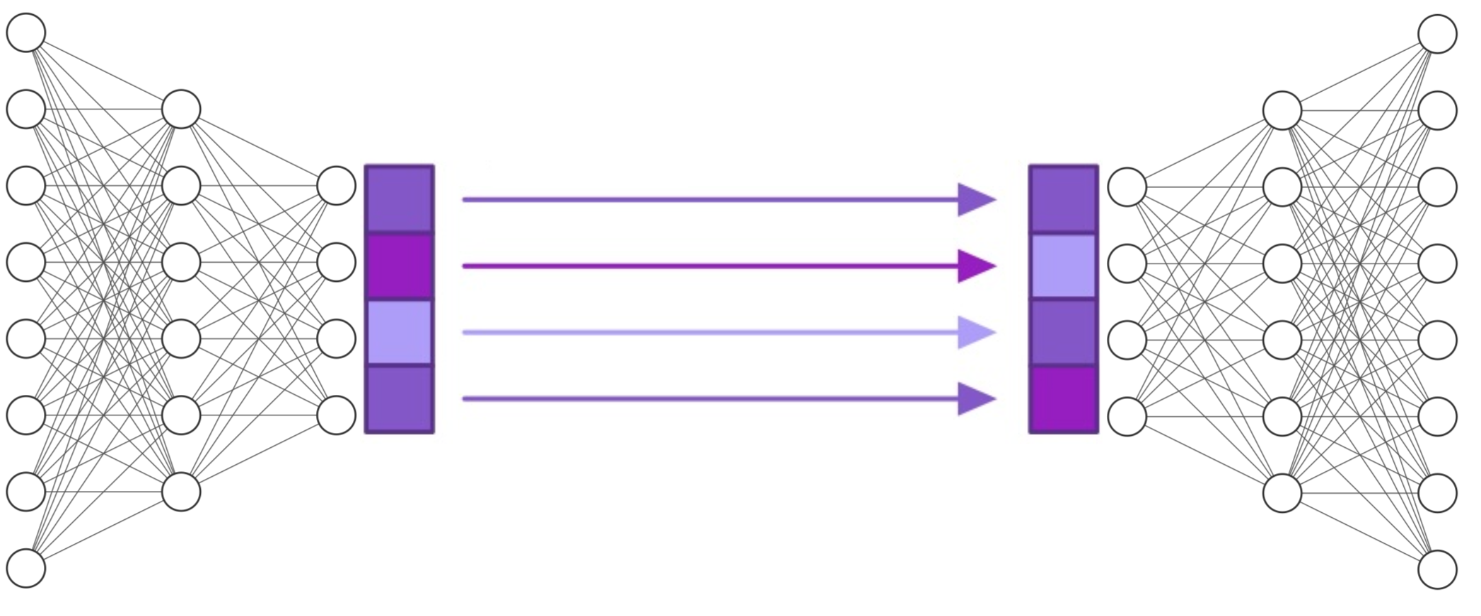
- Latent NeuralODE: NeuralODE combined with an autoencoder.
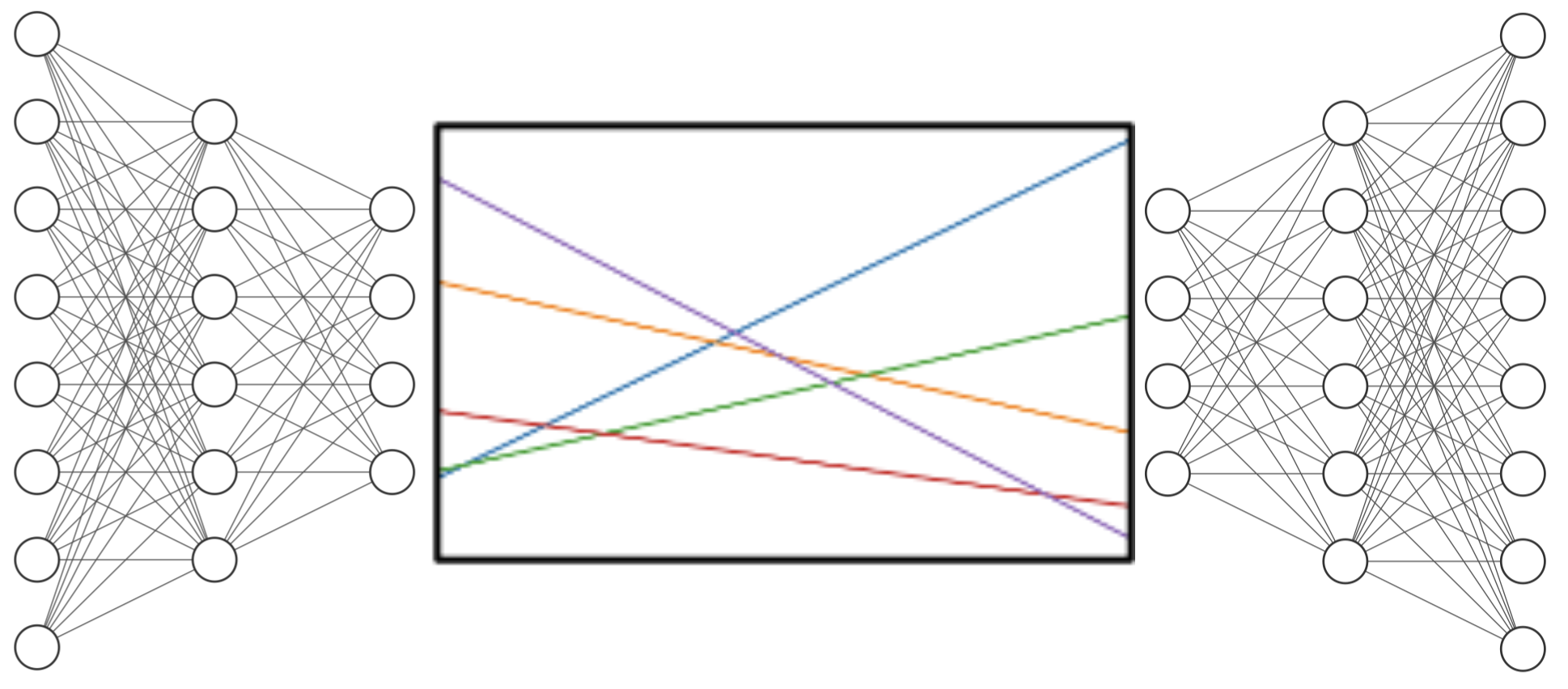
- Latent Polynomial: Uses an autoencoder similar to Latent NeuralODE, fits a polynomial to the trajectories in the latent space.
Find more information on the surrogates below.
Baseline Datasets
The following datasets are currently included in the benchmark:
- osu2008: 1000 samples, 100 timesteps, 29 chemical quantities.
- branca24: 1000 samples, 100 timesteps, 29 chemical quantities.
- simple_ode: 1000 samples, 100 timesteps, 29 chemical quantities.
- simple_reaction: 1000 samples, 100 timesteps, 29 chemical quantities.
- lotka_volterra: 1000 samples, 100 timesteps, 29 chemical quantities.
Find more information on the datasets below.
Plots, Plots, Plots
While hard metrics are crucial to compare the surrogates, performance cannot always be broken down to a set of numbers. Running the benchmark creates many plots that serve to compare performance of surrogates or provide insights into the performance of each surrogate.
Uncertainty Quantification (UQ)
To give an uncertainty estimate that does not rely too much on the specifics of the surrogate architecture, we use DeepEnsemble for UQ.
Interpolation, Extrapolation, Sparsity
Surrogates are often used to interpolate or extrapolate data. The benchmark includes models that are trained on subsets of the training data, investigating their performance in interpolation and extrapolation in time as well as their behaviour in data-sparse circumstances.
Parallel Training
To gain insights into the surrogates behaviour, many models must be trained on varying subsets of the training data. This task is trivially parallelisable. In addition to utilising all specified devices, the benchmark features some nice progress bars to gain insights into the current status of the training.
Dataset Insights (WIP)
"Know your data" is one of the most important rules in machine learning. To aid in this, the benchmark provides plots and visualisations that should help to understand the dataset better.
Tabular Benchmark Results
At the end of the benchmark, the most important metrics are displayed in a table. Additionally, all metrics generated during the benchmark are provided as a CSV file.
Reproducibility
Randomness is an important part of machine learning and even required in the context of UQ with DeepEnsemble, but reproducibility is key in benchmarking enterprises. The benchmark uses a custom seed that can be set by the user to ensure full reproducibility.
Custom Datasets and Own Models
To cover a wide variety of use-cases, the benchmark is designed such that adding own datasets and models is explicitly supported.
Interactive Config Maker
The initial setup can be a bit confusing and the benchmark has many features. To make this easier, we provide an interactive Config Maker that helps to set up the benchmark for the first time. Find it here!
Surrogate Models
The benchmark includes several surrogate models that can be trained and compared. All surrogates
are subclasses to the base class AbstractSurrogateModel, which contains common
methods (like obtaining predictions and saving a model) and mandates the implementation of
some surrogate-specific methods. The following list provides a brief overview of the models and
their characteristics.
-
Fully Connected Neural Network
This is the vanilla neural network, also known as a multilayer perceptron. It is included as the basic model but seems to perform surprisingly well for some cases. The inputs are the initial conditions and the time where the solution is to be evaluated. -
DeepONet
DeepONet consists of two fully connected networks whose outputs are combined using a scalar product. The trunk net receives as input the initial conditions, while the branch net receives the time where the solution is to be evaluated.
In the current implementation, the surrogate is a single DeepONet with multiple outputs (hence it is referred to as MultiONet in the code). This is achieved by splitting the output vectors of branch and trunk net into multiple parts. Corresponding parts of the output vectors are then combined using a scalar product. -
Latent NeuralODE
Latent NeuralODE combines NeuralODE with an autoencoder. The autoencoder reduces the dimensionality of the dataset before solving the dynamics in the resulting latent space, making it an efficient and powerful surrogate model. -
Latent Polynomial
This model also uses an autoencoder similar to the Latent NeuralODE, but instead of solving differential equations, it fits a polynomial to the trajectories in the latent space. This approach offers a different trade-off between complexity and accuracy.
Data
This page provides an overview of the five datasets included in the benchmark. Click on any dataset name below to expand and see for a description and plots. For a full explanation of data structure, configuration, and how to add your own datasets, see the documentation below.
coupled_oscillators
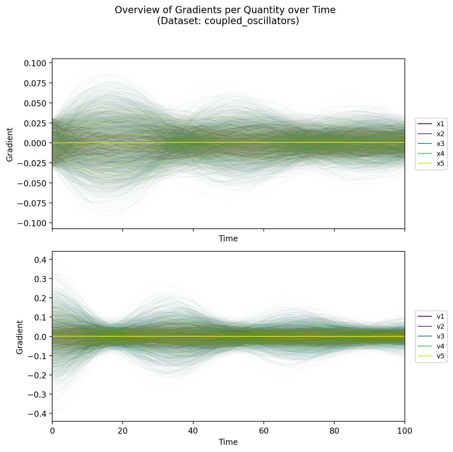
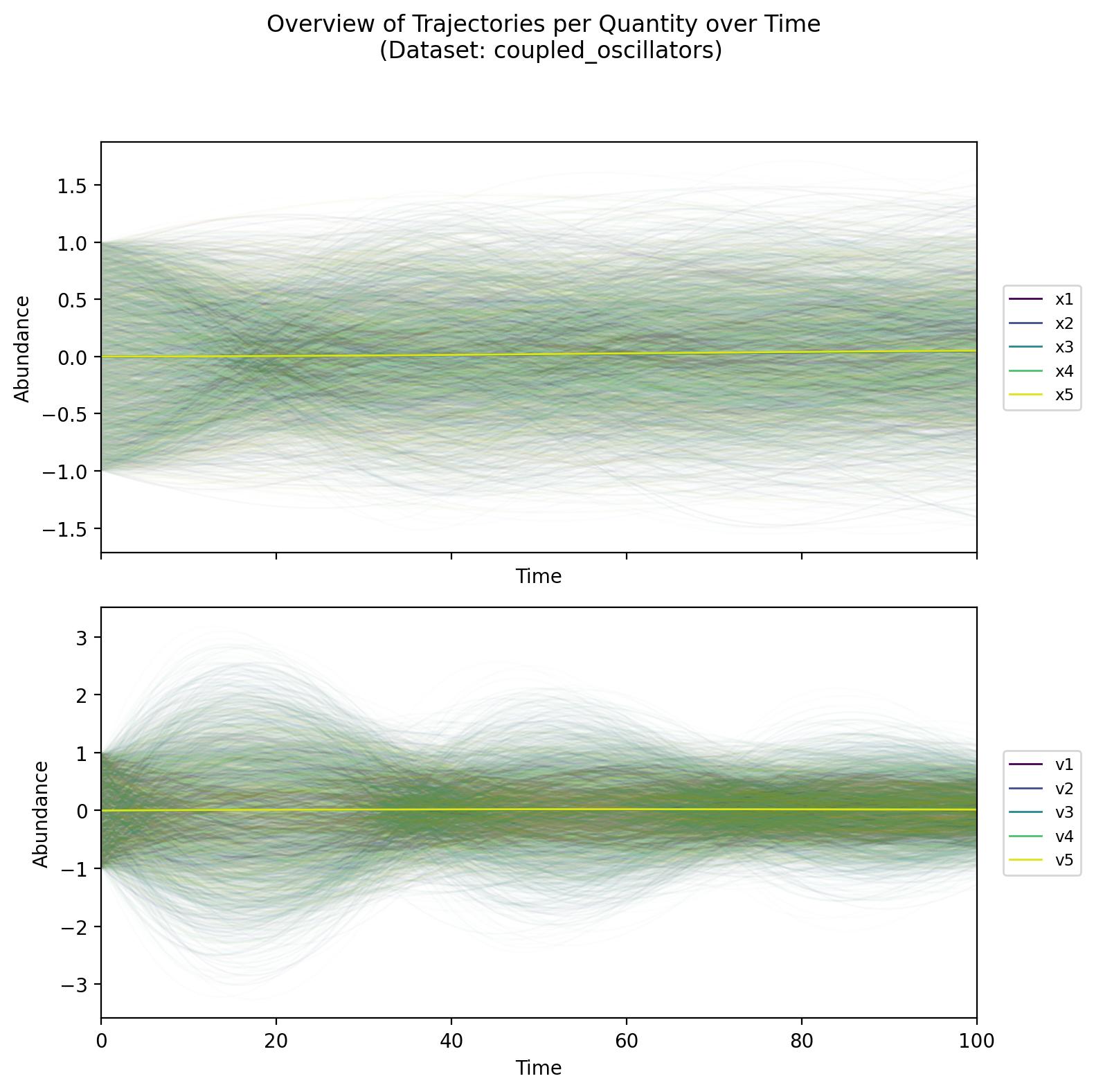
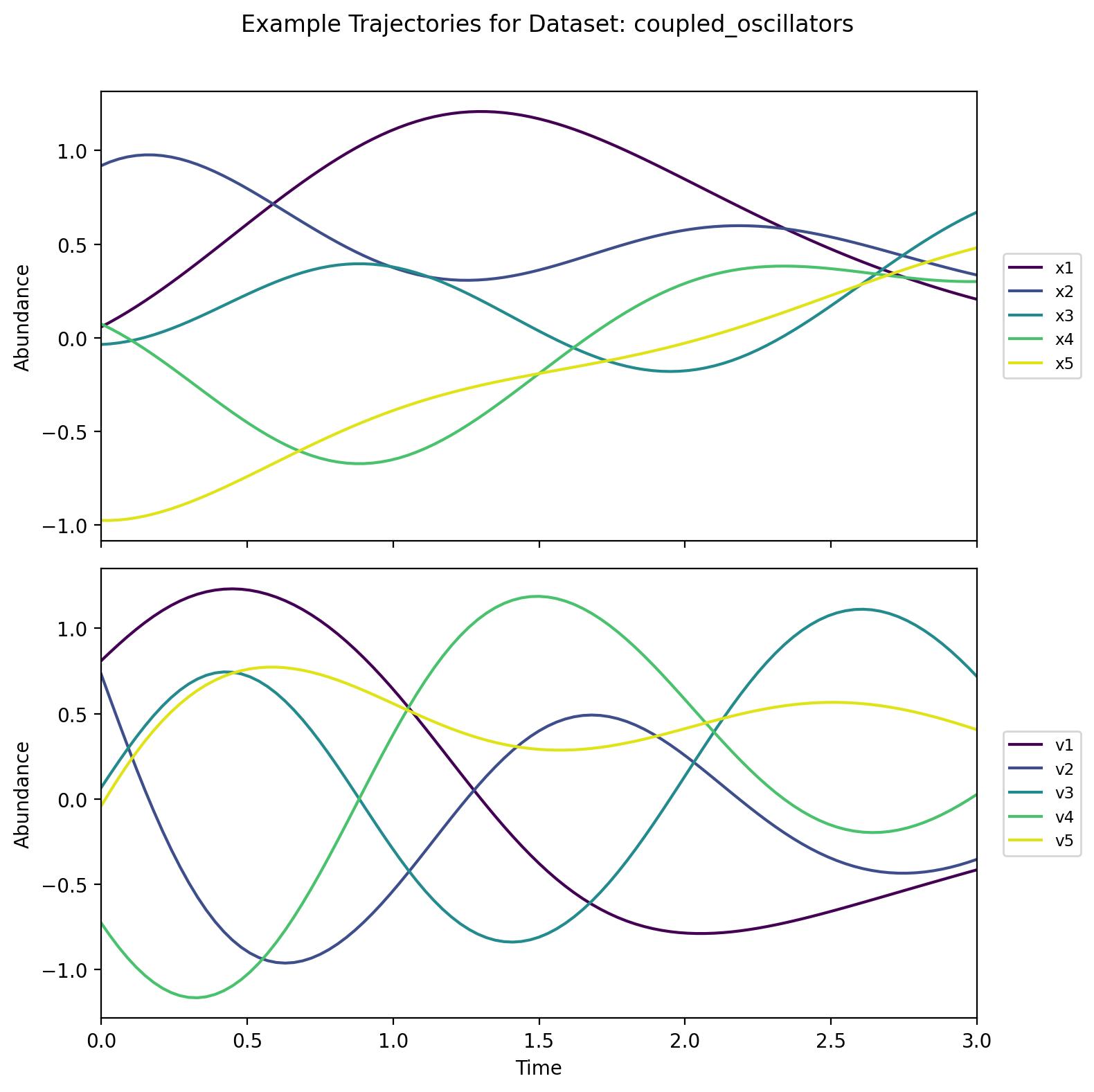
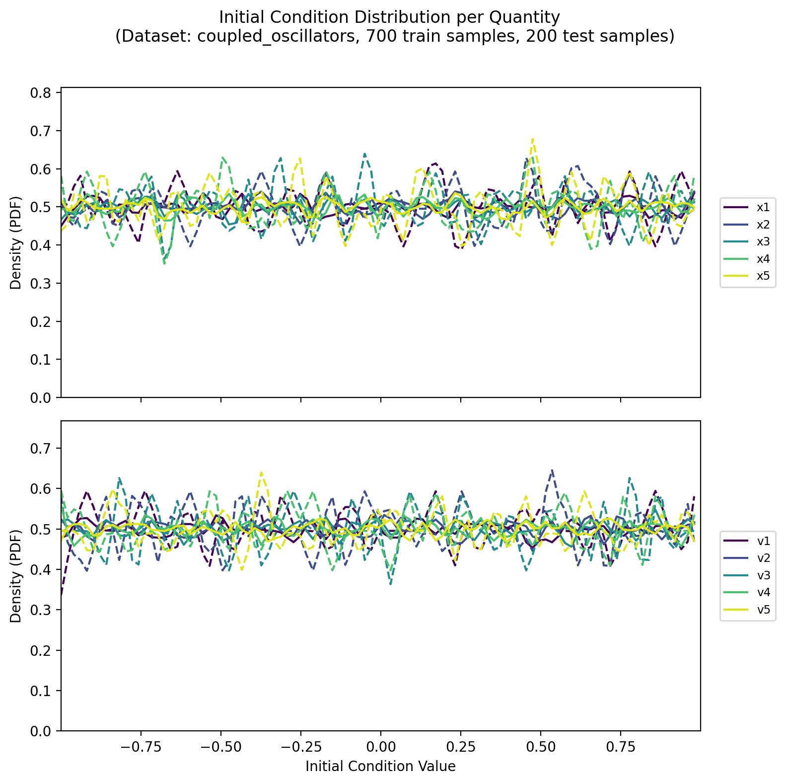
A system of five oscillators (each with position and velocity) coupled through both linear and non-linear spring forces. Unlike the other datasets, the quantities here can be negative, and the trajectories are best kept in linear space rather than log space. This setup highlights interactions between multiple oscillators and demonstrates more complex dynamics due to the non-linear coupling terms.
lotka_volterra
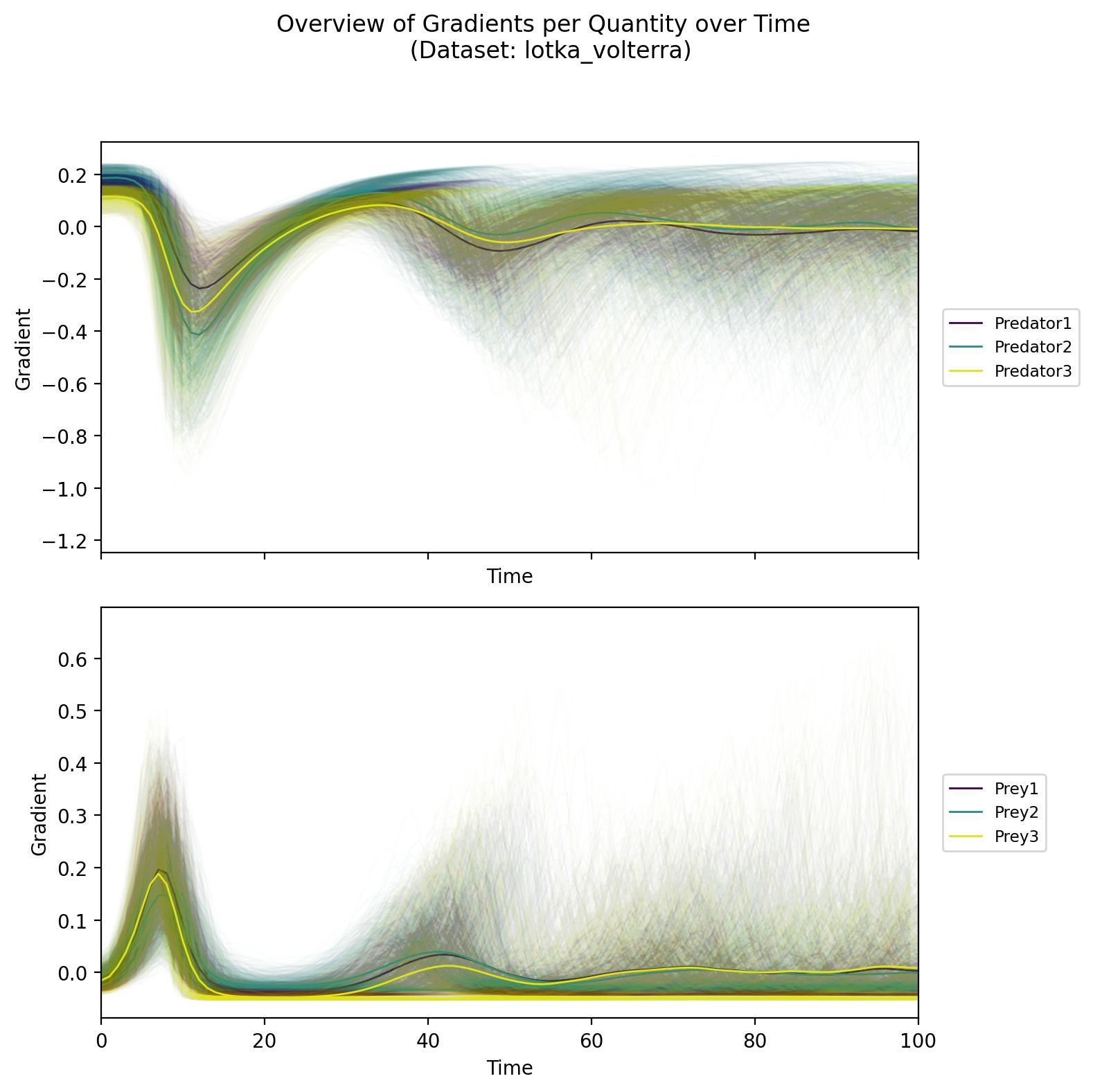
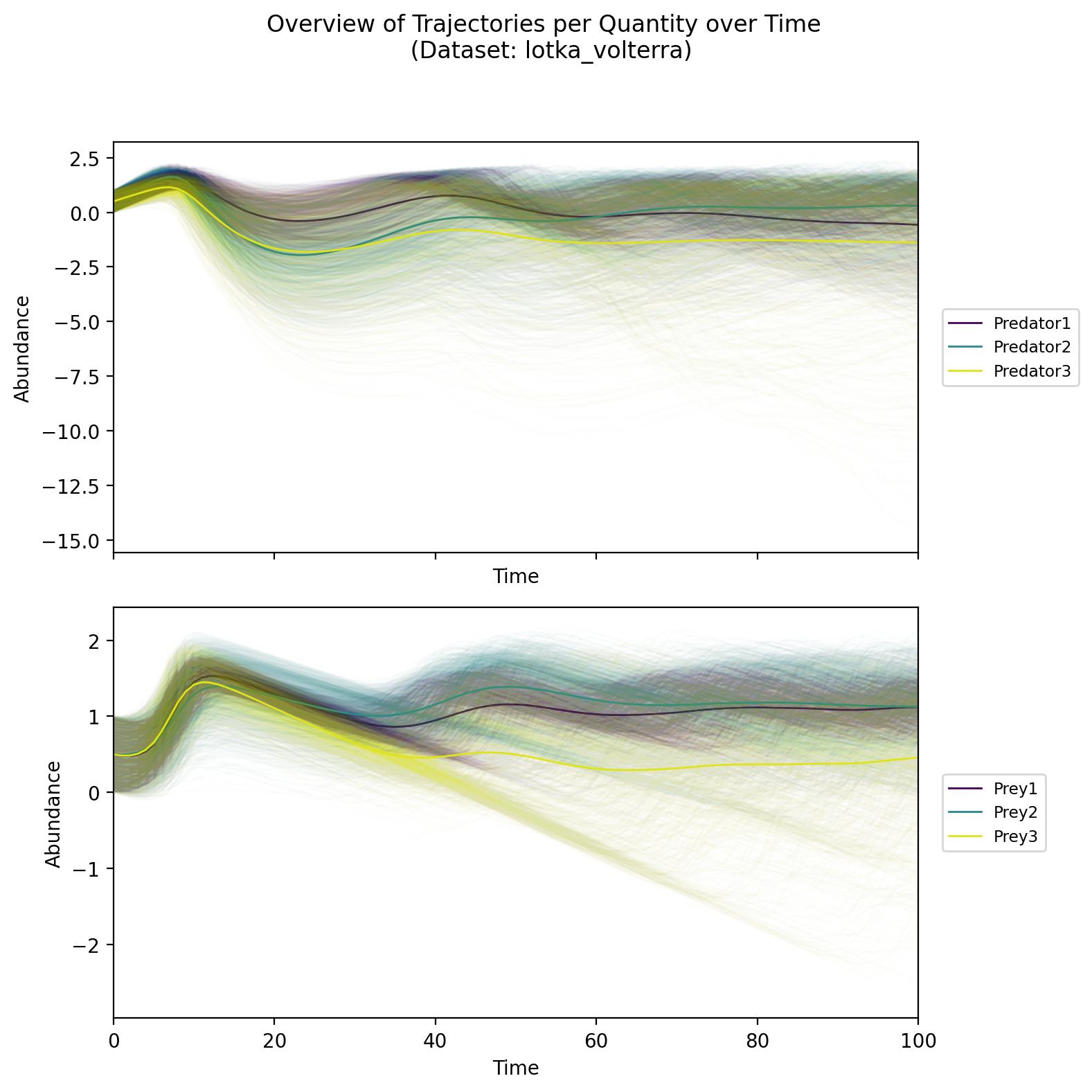
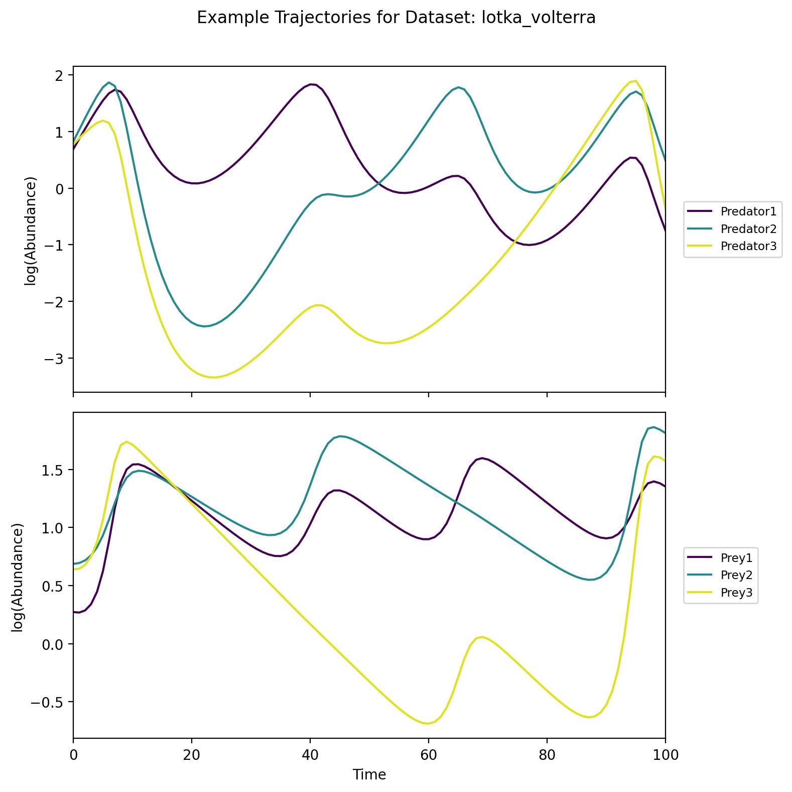
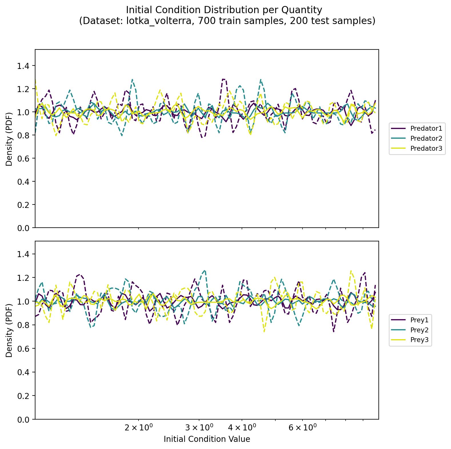
An extended predator-prey model with six interacting species—three predators and three prey. Certain initial conditions can lead to populations spanning multiple orders of magnitude, resulting in cyclic or complex population dynamics. This dataset highlights both cyclical interactions and substantial variability across different initial conditions.
osu2008
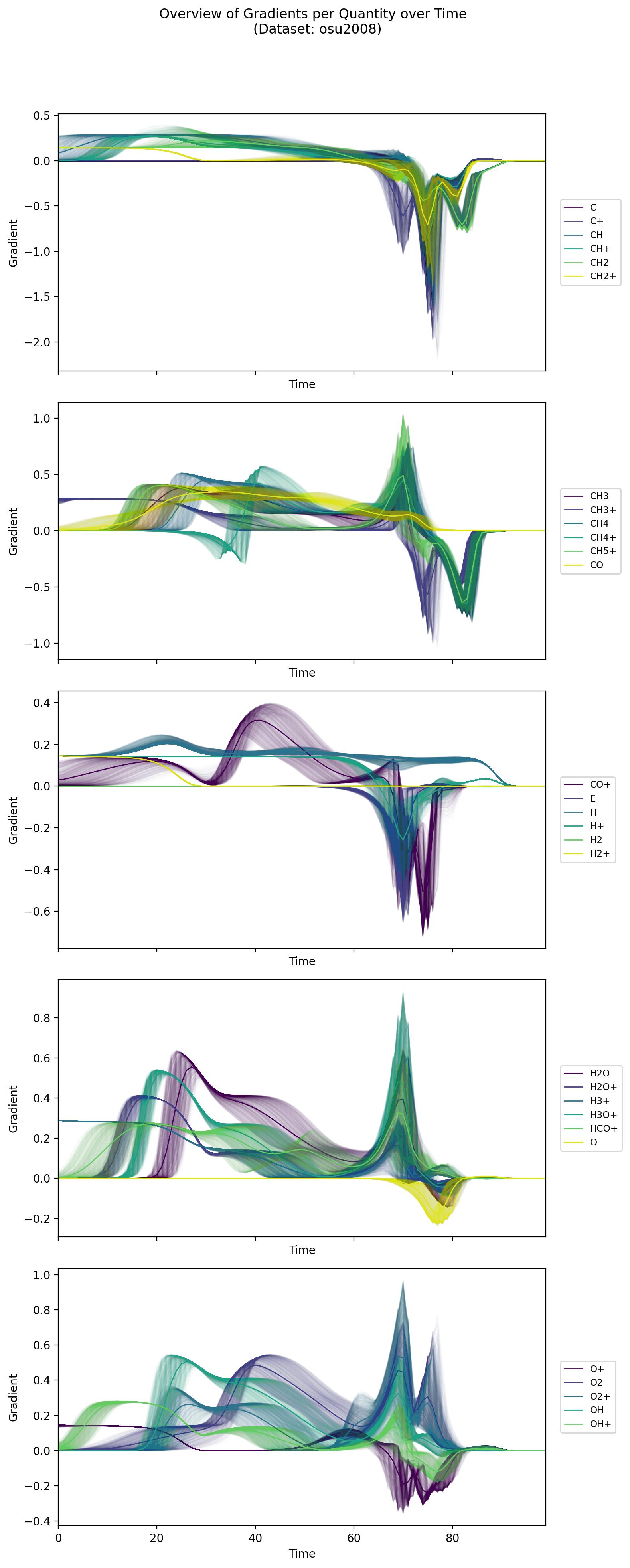
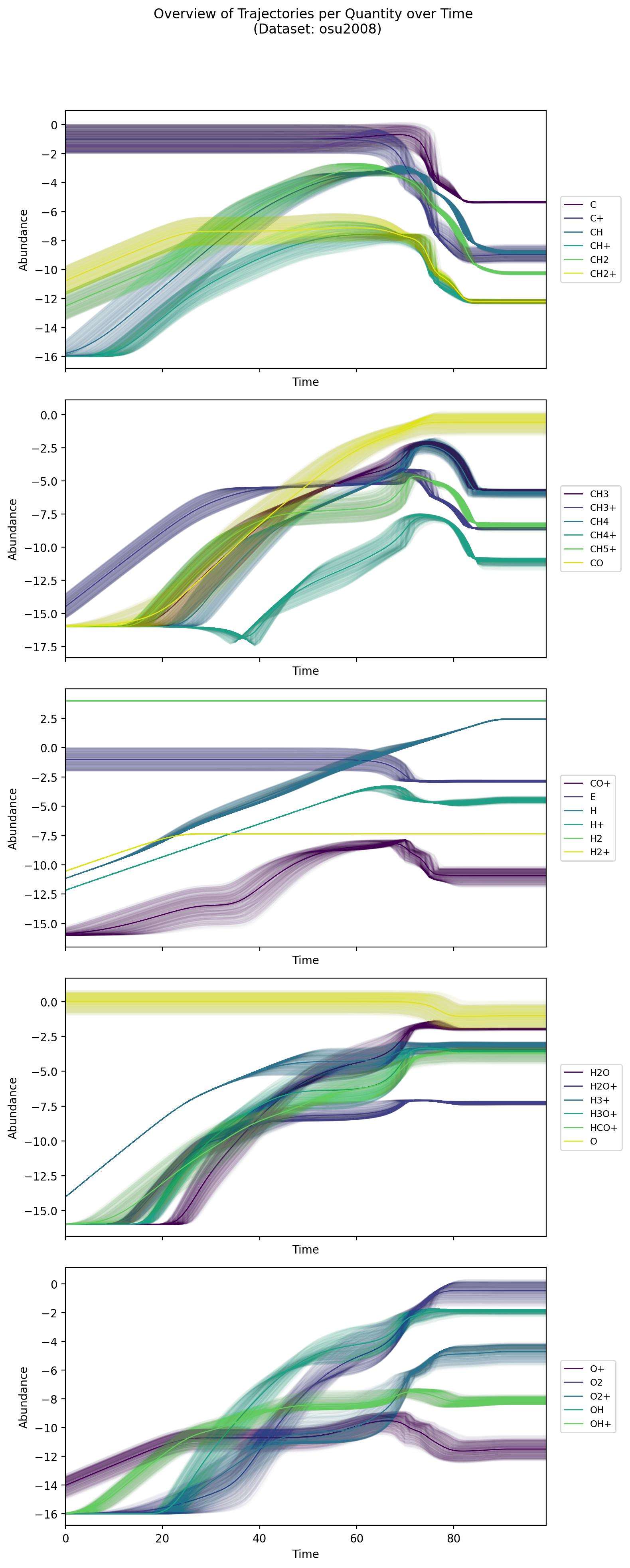
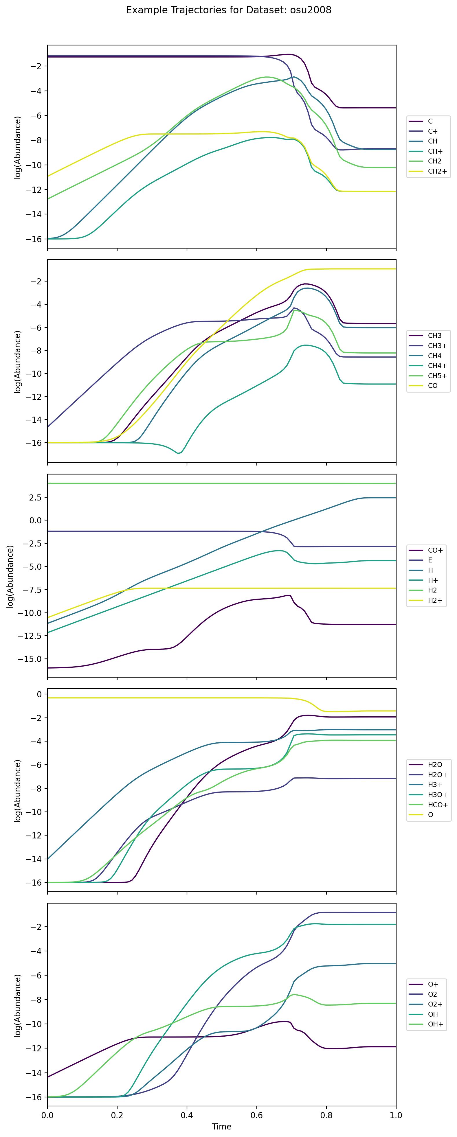
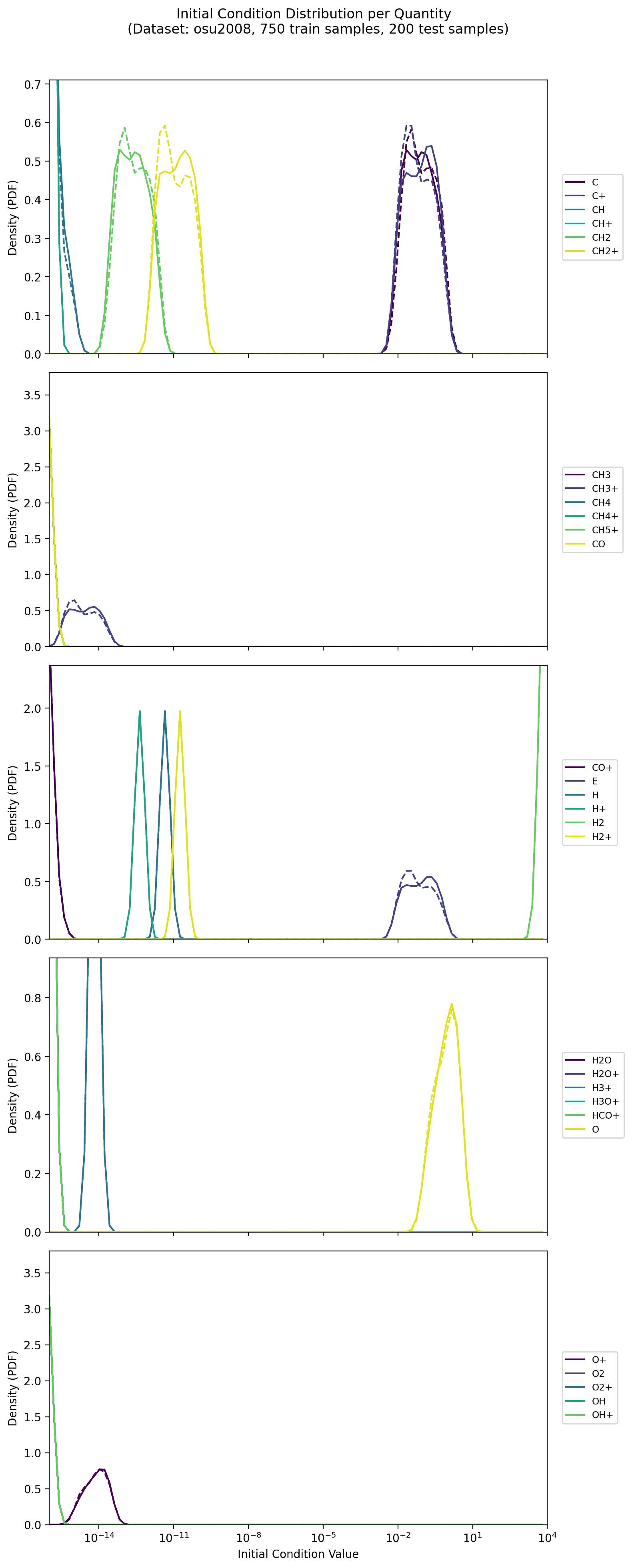
Derived from an astrochemical reaction network of 29 chemical species, this dataset covers a wide range of timescales (up to 10^8 years) in log space. Its initial conditions are generated through a specialized procedure that sets floors and bounds for key species. The complexity and scale mirror real astrochemical processes, making it more intricate than simpler toy examples.
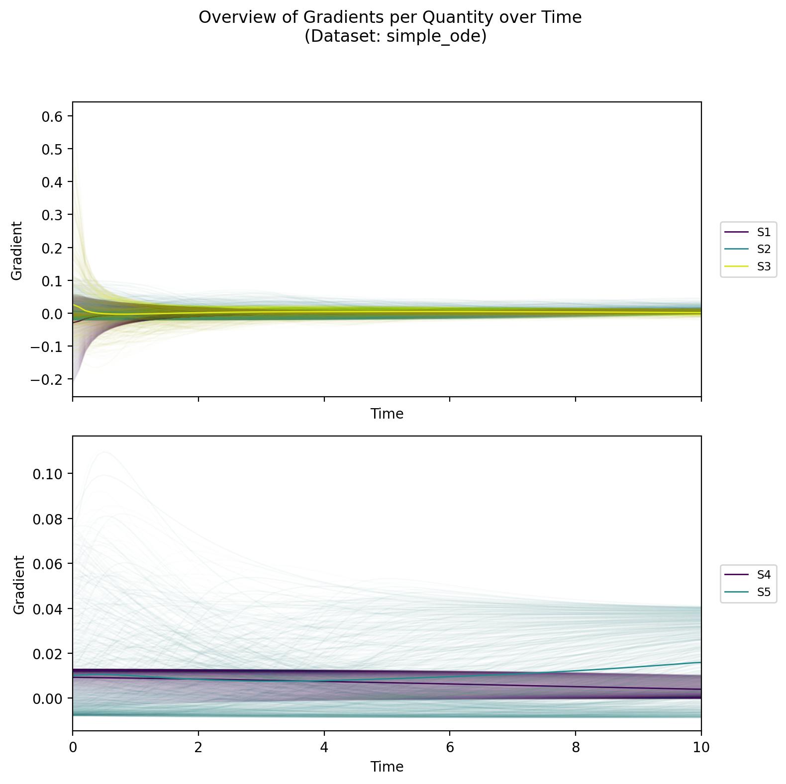
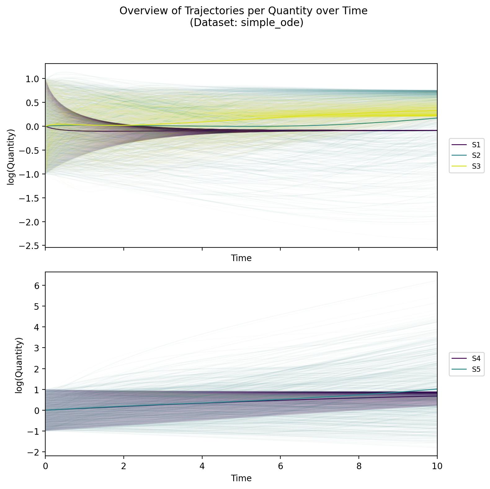
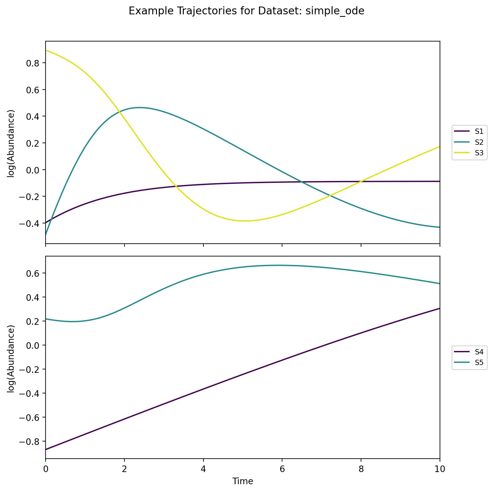
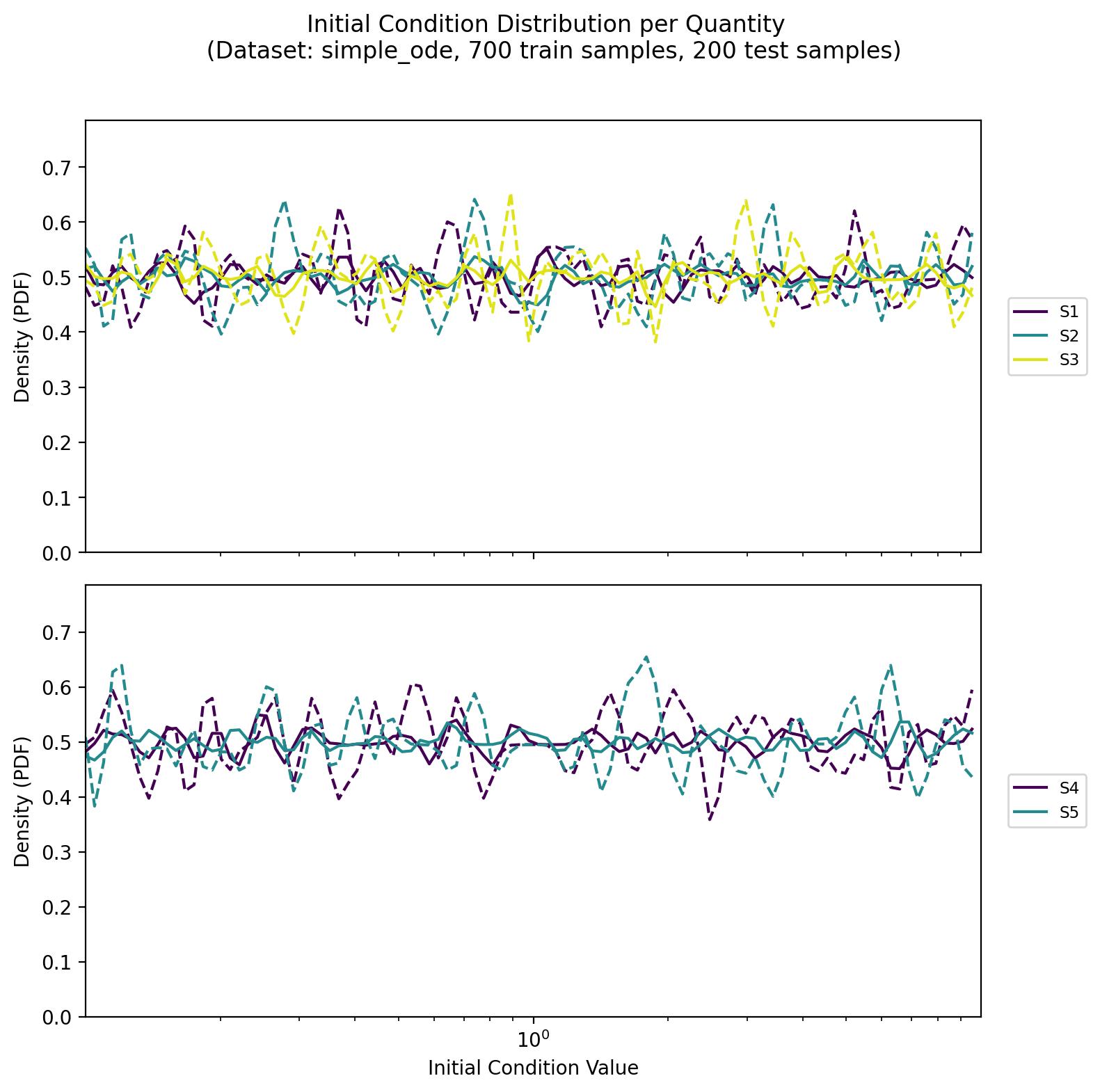
simple_ode
A five-species system with soft non-linear effects and non-conservative behavior. Each species has logistic-like self-regulation combined with interactions among them. Although smaller than the astrochemical examples, it still showcases interesting population dynamics and the interplay of internal regulation with cross-species effects.
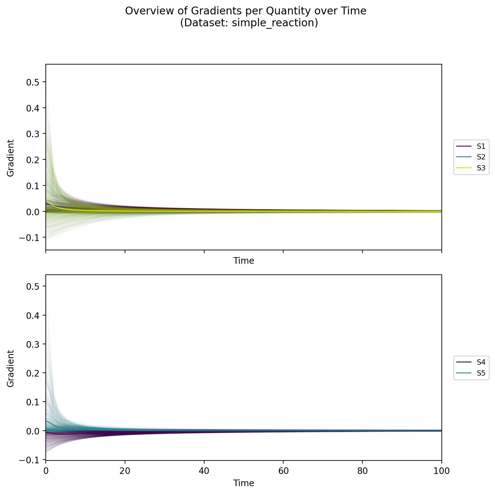
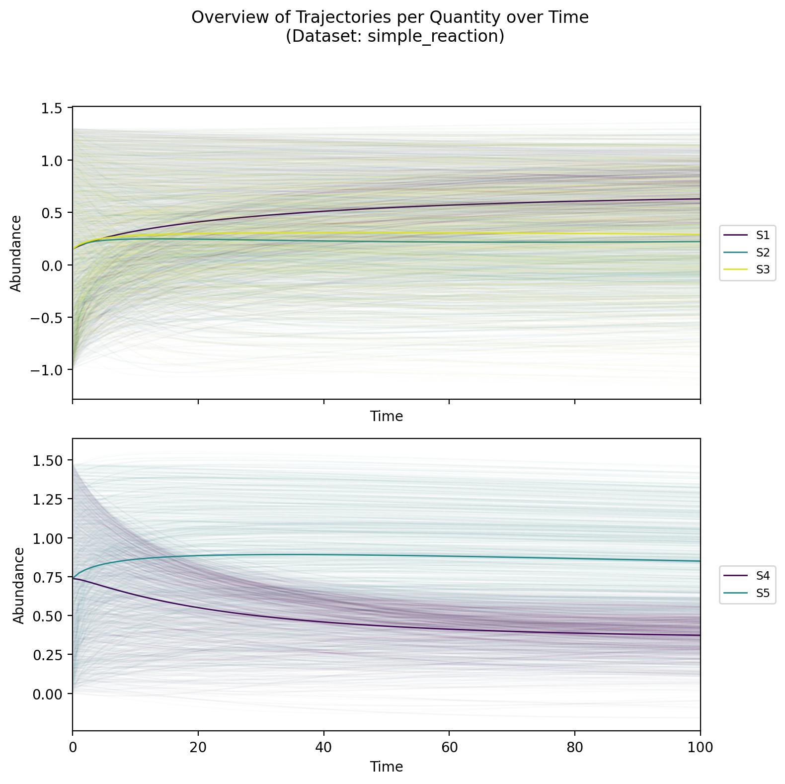
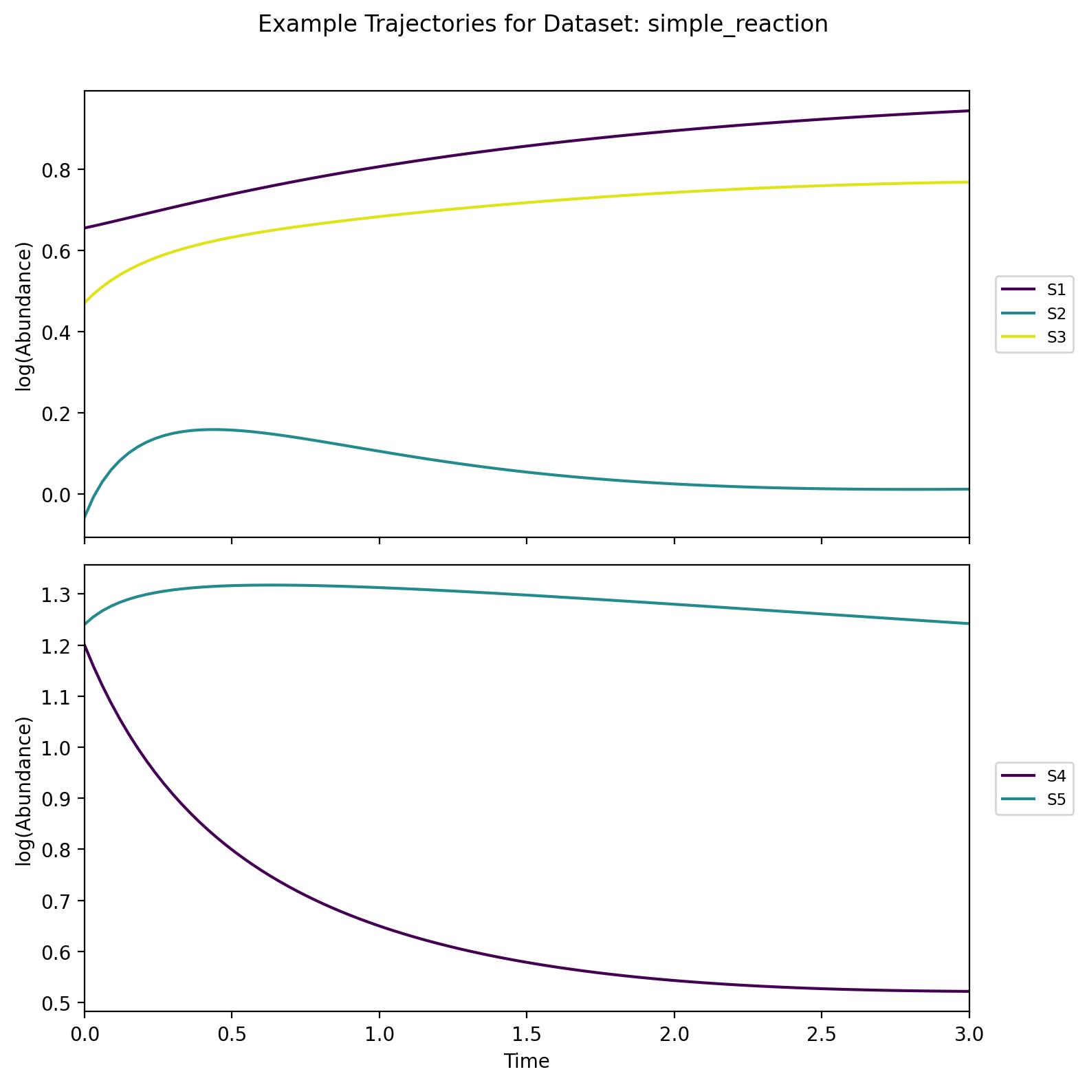
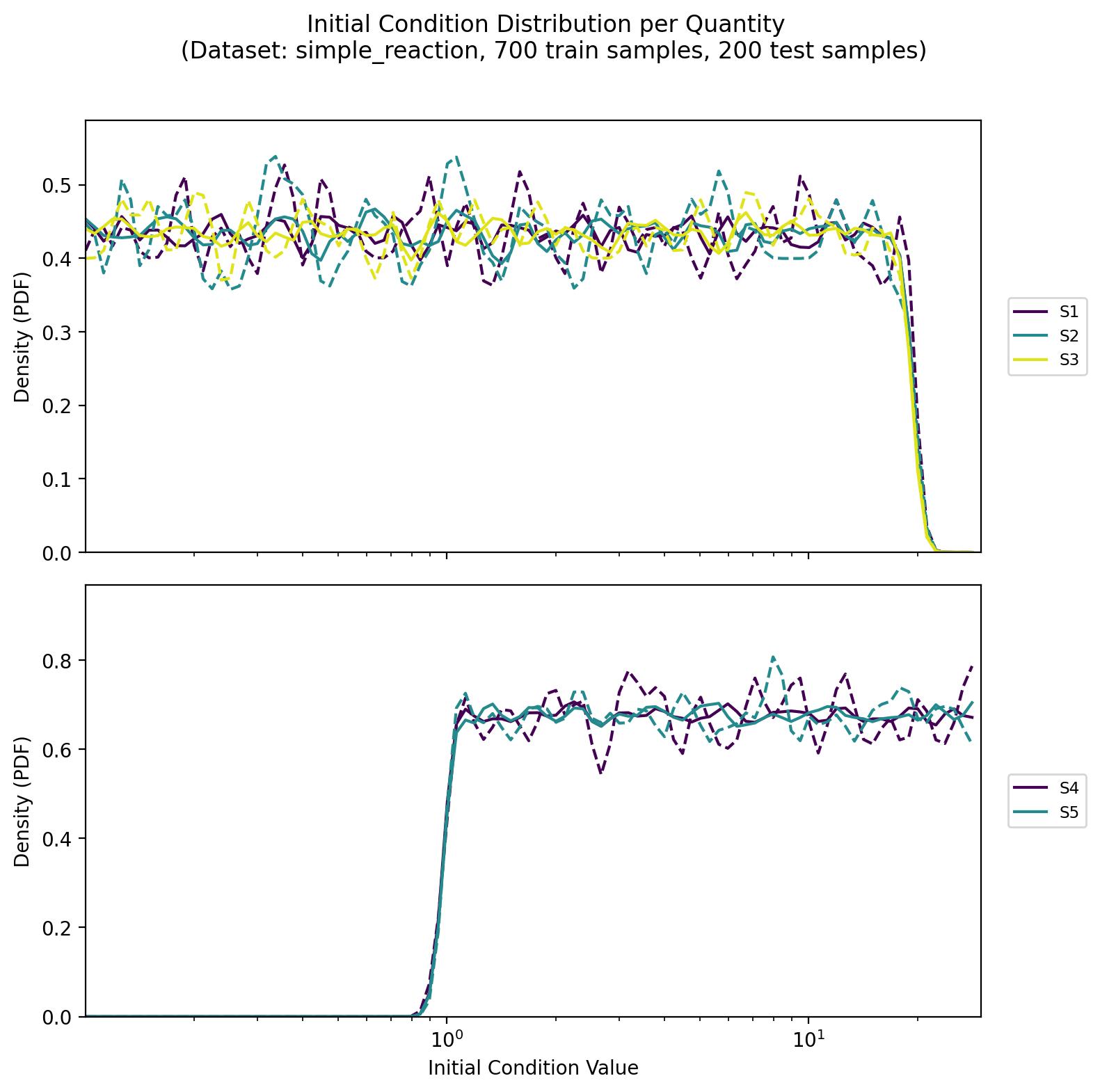
simple_reaction
A five-species chemical network involving both reversible and irreversible reactions, sampled in log space for each species. Despite being simpler than the astrochemical network, it incorporates realistic reaction kinetics (mass action) with quadratic and linear terms, capturing essential features of chemical reaction systems in a more compact form.
Data Structure
All datasets are stored in the datasets folder in the root directory. A dataset can
be
identified
by
the name of its folder - the directory containing the osu2008 dataset is
datasets/osu2008/.
Inside this folder, there is a file data.hdf5, which contains the data as well as some
metadata.
The data is already split into training, validation and test data. This split depends on how
the
dataset is created, we recommend 75/5/20 %. The training data (or subsets thereof) is used
to
train the models, the validation data is only used to compute a slightly more represantive
loss
and accuracy during training, hence it can be rather small (and should be for performance
reasons, as the losses and accuracies are computed every epoch). The test data is then used
for
the actual benchmark.
Model Configuration
Additionally, the dataset folder might contain a file surrogates_config.py. This file
contains
dataclasses that specify the configuration of each surrogate for the given dataset. While it
might
be the case that the base configuration (which is stored in the config file in the folder
surrogates/surrogate_name/) is sufficient, usually the hyperparameters of a model must be
adjusted
for each dataset to achieve optimal performance. This can be done by creating a dataclass in
surrogates_config.py. The dataclass should have the name surrogate_model_name + "Config"
(e.g.
MultiONetConfig). It is sufficient to specify parameters here that deviate from those set in
the
base class. As an example, if we want to reduce the number of layers in our fully connected
network, we simply add num_hidden_layers = 4 into the
FullyConnectedConfig dataclass.
The
benchmark will then use these parameters for the model on this dataset.
Adding a Dataset
Adding a new dataset is pretty easy. The only requirement for the dataset is that it should
be a
numpy array of shape
[num_samples, num_timesteps, num_chemicals]. The
technical
details can be found in the documentation. The
benchmark supports one big numpy array or three separate arrays if you already have a custom
split. Since the quantities often span many orders of magnitudes, the surrogates will
usually
train on and predict normalised log-data. It is recommended to add the data "raw", the
benchmark
takes care of the log-transformation and normalisation (but it can also handle data that is
already in log-format). Optionally, you can provide the corresponding timesteps and labels
for
the quantities in the dataset, these will then be used for visualisation.
Training
To ensure a fair benchmark, it is important that the surrogate models involved are actually
comparable, meaning they are trained under similar circumstances and on the same training
data.
For this reason, the benchmark involves training the models before comparing them (rather
than
simply benchmarking models previously trained somewhere else).
There is already some application-specificity involved in choosing for how long to
train the model - usually, we want to compare best-performing models, which means training
each
model for as long as it reasonably keeps converging. But if low training time is essential
(e.g.
for fast re-training), one could also choose to train all models for equal amounts of time
or an
equal number of epochs.
Configurations
In the following paragraphs, you can find detailed explanations on the config settings and how they are relevant for the training. For an easy way of making a config file that conforms to the requirements of the benchmark, head over to our Config Maker!
The training of the models is configured in the config.yaml file (even more details
on the config here). A benchmark run is identfied by a
training_id. The surrogates to be included in the benchmark can be
provided in the form of a list of strings, where the strings must match the names of the
surrogate classes (e.g. ["FullyConnected","DeepONet"]).
The epochs and batch_size parameters are used to specify the number of
epochs to train the models and the batch size to be used during training, hence one value per surrogate is required. They should be provided as a list of integers, where the ordering corresponds to that of the names of the surrogates. The benchmark
will train each model for the specified number of epochs and with the specified batch size.
The name of the dataset to be used is
specified in the
dataset section, along with the option to log-transform the data, specify how to
normalise it, whether to use_optimal_params that were determined in previous hyperparameter tuning
and which tolerance to use for small values.
The device parameter specifies the device(s) to be used for training. They can be
specified as a list of strings (e.g. ["cuda:0","cuda:1"]), where each string is the
name of a device. The devices must be available on the machine and support PyTorch. The
benchmark will use all devices specified in the list for training, more on this in the parallel training section.
The seed parameter is used
to ensure reproducibility of the training process. The seeds for all models are generated from
this seed on a per-task basis.
The verbose will toggle some additional prints, mostly during the benchmarking
process.
Besides training one main model on the provided training sets, many additional models will be trained depending on the configuration of the benchmark. These models are required to investigate the behaviour of the model under various circumstances:
- Interpolation: If this mode is enabled, one additional model will be trained per
interval
specified. The train set for this model will be "thinned" in time using numpy array
slicing,
i.e.
train_data = train_data[:,::interval,:]. This means that only every n-th timestep will be given to the model during training, but during testing it will be evaluated on all timesteps, including those in between the provided timesteps. - Extrapolation: If this mode is enabled, one additional model will be trained per cutoff
specified. The train set for this model will be trimmed in time using numpy array
slicing,
i.e.
train_data = train_data[:,:cutoff,:]. This means that the model is only trained with timesteps up to this cutoff, but must later predict the trajectories for all times. - Sparse: If this mode is enabled, one additional model will be trained per fraction
specified. The train set for this model will consist of fewer samples than the original
training data, obtained using
train_data = train_data[::fraction,:,:]. This means that only every n-th sample will be given to the model during training. - Batch Scaling: If this mode is enabled, one additional model will be trained per batch size specified. The model will be trained with the specified batch size. This can be useful to investigate the effect of batch size on the model's accuracy or inference time.
- Uncertainty: If this mode is enabled,
n_models - 1additional models will be trained on the full dataset (since the main model can be used in the DeepEnsemble too). Each model will be trained with a different random initialisation and a shuffled training set. Together they form a DeepEnsemble, which can be used to estimate the uncertainty of the model's predictions.
Lastly, there are some settings that do not influence the training process. The parameters
gradients, timing, compute, losses and
compare are only relevant for the benchmarking process, they will either toggle
additional evaluations of the main model or further output based on existing data.
Parallel Training
To reduce the potentially long training process due to the large number of models, the
benchmark
is parallelised. The benchmark will utilise all devices specified in the config file to
train
the models. The parallelisation works simply by creating a list of all models to be trained
("tasks") and then distributing these tasks to the available devices. A progress bar will be
displayed for each training in progress as well as for the total progress. In principle one
can
also train multiple models on the same device, simply by listing it multiple times:
["cuda:5","cuda:5"]. Whether this has any benefit depends on the model and
device.
Of course, it is also possible to train sequentially using a single device only.
The task-list approach has two benefits: It is asynchronous in that each device can begin
the
next task as soon as it finishes its current task, and it makes it easy to continue training
the
required models at a later time in case the training process gets interrupted.
Saved Models
After the training of each model finishes, it is saved to the directory
trained/training_id/surrogate_name (e.g. trained/training_1/FullyConnected/). The
model names are specific to the task and may not be changed, as the later parts of the benchmark
rely on loading the correct models and models are primarily identified by their name. For each
model, two files are
created, a .pth file and a .yaml file. The former not only contains
the model dict with the weights, but also most attributes of the surrogate class, while the
latter contains the models hyperparameters as well as some additional information (information
about the dataset, train duration, number of training samples and timesteps, ...).
Benchmarking
After the training finished, the models are benchmarked. Similar to training, it is important to
treat all models equally during the benchmarking process. This is not trivial, as the models
have different architectures and may require differently structured data. The benchmark attempts
to equalise the process as much as possible, hence the requirements for implementing additional
models are relatively strict.
One example of this is that the predict method of the surrogate class is the same
for all models, i.e. it is implemented in the abstract base class
AbstractSurrogateModel. For this to work, each model must have a
forwardmethod that conforms to certain standards. More details on this can be found
in the documentation.
The below sections describe the structure of the benchmark and how to configure it. For precise accounts of the evaluations and plots made by the benchmark, head to the next section, Output.
Structure
The general structure of the benchmark is that the models are first benchmarked indivdually and
then compared to one another.
The individual part mostly consists of obtaining predictions
for
the trained models on the test set and comparing them to the ground truth. The results for each
surrogate are used to make surrogate-specific plots, which are stored in the
plots/training_id/surrogate_name/ directory. In addition, these results are stored
in one large
nested dictionary, which roughly conforms to the structure
metrics[surrogate_name][category][metric].
This dictionary is the foundation for the
comparative
part, which creates comparative plots as well as tabular output. The results -
.yaml files for each surrogate, a metrics.csv file and
metrics_table.txt are stored in results/training_id, while the plots
are stored in plots/training_id/.
Configurations
Below there are explanations on how the config settings are relevant for the benchmarking. For an easy way of making a config file that conforms to the requirements of the benchmark, head over to our Config Maker!
The benchmarking of the models uses the same config.yaml file (more details
here) that is also used to configure the training. It is
recommended to use the configuration that was specified during training for minimal
complications, but it is also possible to change many of the configuration parameters.
The models for the benchmark are identified by the
training_id, and the ID is also used to make directories in the plots/
and results/ folders. The dataset section should remain untouched, as
the training is always dataset specific. It is possible to remove surrogates for
the benchmark that were included in the training (but not vice-versa, since you cannot benchmark
surrogates for which no models were trained). The dataset section should remain
untouched, as the training is always dataset specific. The benchmarking process is not parallel
since it is much faster, so only one device is required. If multiple are specified,
only the first one in the list will be used. Similarly, the seed is not relevant
for the benchmarking process, as the models are already trained. If you want some additional
information, use the verbose parameter.
The logic of the surrogates also applies for the different modalities of the benchmark - if they
were included in the training, they can be removed for the benchmark, but you can not add
modalities that were not included during training. It may be possible to reduce the details for
each modality the benchmark (i.e. to only use intervals 2-5 when you trained with 2-10), but
they best remain untouched.
The parameters losses, gradients, timing and
compute toggle the respective evaluations of the models. Since they do not change
anything about the training process, they can be toggled freely.
Lastly, the compare parameter
determines whether the models are compared after benchmarking them individually. It is not
possible to run only the comparative part of the benchmark, as the individual benchmark results
are required before the surrogates can be compared! If only some modalities of the individual
benchmarks were run, the models will only be compared for these modalities (e.g. there will be
no comparison of the extrapolation performance of the models if
extrapolation = False). All details about the outputs and results of the benchmark
results are listed in the Output section. The next section will give an
overview over
Modalities
WIP